Tuesday, 25 November 2008

Roland Levinsky Mapping

Since last week I have obtained the Blue tooth data of the Roland Levinsky Building as I explained in my last post and have then mapped it out accordingly. The map I produced is as follows:

This map displays all the Blue tooth devices found, relating to which floors they were available on. I chose to focus on this element of the data as it was quite interesting how some devices were available only on one floor while others were multi-floored. However it was difficult to tell from the data which ones stretched over how many floors and so I incorporated this into my map of the building to create a better visual representation by which the data could be more easily understood. The image has a key as well as showing the floor numbers down the side as this enabled the data to be split up more precisely and to be grouped with devices that showed similar characteristics.

The next step in this project is to start to use GPS to map environments more accurately.

Tuesday, 18 November 2008

Hertzian Space

Last week we were asked to map the hertzian space of an area as the start of a project into Hertzian space for IDAT106. For this task I decided to map the wifi networks in Alexandra Works, the student accomodation which we are staying in. I chose this as I have a wifi network in my room, and I was intrigued to find out how many other people had decided to do the same as me, especially being that sharing networks is disallowed in the building. I therefore downloaded some stumbler software and took my laptop around the building with a floor plan for each floor to find all the wireless networks and log what I found. The results of this were quite surprising as I found at least 30 networks in the building which only has around 45 cluster flats, meaning that almost every cluster flat has at least one wifi network within it. Below is the list I accumulated from this and then the prototype map I made from the data I could use:


When producing the prototype map on paper for this I chose to use circles to resemble the edge of the area which the network could be reached within. The networks themselves are not shaped in an exact circle, due to the effect of walls and other objects which cut through the space, but I decided that, theoretically, without those obstacles the network should be basically cirular. This also enabled me to map the networks as their distorted shape would be very difficult to define with the technology I have available. I also layered all of the floors on top of each other so that the networks were seen from a birds eye view.
Once I had drawn this, I decided I would translate the prototype to a 3D image so that the idea of a spherical boundary within which a network is available could be more easily portrayed. This image I colour coded similar to that of the 2D map above to demonstrate their relation. Below is this image from 4 different angles in this order (front, back, left, right):


I then showed this to my IDAT106 tutor who suggested that in its current state the 3D map was difficult to understand and read as there was no information explaining what was what and where within the space. I may have been able to understand the image because I knew the space but no one else did and so better communication of the image was needed. I therefore drew up the following image to help solve this:

I could also have chosen to place the floor plan of the space onto this image in relation to the wifi spheres to give a better understanding of the layout, but the angles needed for this would make the image more difficult to read and so I stuck with just displaying where the levels were for each floor in relation to the networks.

The next step for this project is to use GPS to further investigate the hertzian space of the chosen area. I am therefore going to re-do this project in order to make this more accessible for me as the location I have chosen is 20 minutes away from my lectures and so I feel it would be quite difficult to do the GPS mapping efficiently. I am instead going to do another map of the Bluetooth that can be found in the Roland Levinsky building of the university. When I begun this project I had an interest in studying Bluetooth but instead tried to go for something more obscure. By doing the project again in the Roland Levinsky building with Bluetooth, it will make the GPS part of the project more achieveable whilst developing my knowledge further of the hertzian space.

Sunday, 2 November 2008

Final Notations

As I have now completed all of my notations, this post is to show the final completed version of my map of the Picnic with all five notations - time, movement, quiet/noise, hard/soft and dark/light plus the sculpture notation of the hand cast that I made:


I am happy with this overall outcome as it is very dynamic and readable image. The next and final step for this project is to print this image onto A3 paper without the collage background and then work the paper into a 3D surface according to the notations which I have used. By doing this I will be turning something that I have converted into 2D (the Picnic) back into something that is 3D therefore partially returning it to to its original state but in a different form to that which it begun. This could be defined as the Picnic mat to the original Picnic, as the mat is where all the above observations are made, and this final A3 version of my notations will in some ways mimic this scenario. The only aspect missing to make these notations match the Picnic scenario that originally occurred is the aspect of time. Time passed during the original picnic, but this image is static through time and so does not replicate the environment fully.

Hard and Soft is Complete!

Over the last few days I have been researching different ways to illustrate hard and soft to give me inspiration for my own notation of hard and soft in my collage. A lot of the notations I found to begin with were using colour to demonstrate hard and soft surfaces, such as this one:


(http://sofia.usgs.gov/publications/reports/rali/images/10mapx.jpg)


However I do not want to use colour in my notations as this is a less abstract way of displaying the information and may also make my notations unbalanced, as a colour notation may stand out more than the other black line notations I have used and so would draw the viewers attention away from the other information that is provided. The next step I decided to take was to re-define my search so that it was based around density. This is because the density of an object establishes whether an object is hard or soft and so by using this as a measure hard and soft areas could be defined. I therefore started to research into ways of graphically representing density and found this image:


(http://www.optimaldesign.com/AMHelp/Images/density.jpg)


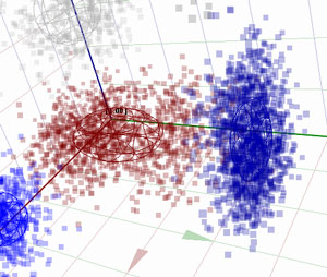
This is a 3D density graph of a cluster of genes. This may not be directly linked to the density of which I refer, but I did feel that this was an interesting image, and also a logical way of displaying density - by replicating the scenario using dots which resembles the particles of the object. I decided to use this idea to notate the hard and soft areas of my collage and so went back to my image and added this final notation:

Key


Notation with image

Notation alone


I am quite happy with this notation as it is easy to understand and deduce information from. This therefore completes my notations. Check my next post for a final overview of what has been created.